Overview
We've done a lot of buildup to get to this point. One thing we haven't done is talk about how this is going to be musical, though. Dumping magnitudes from FFT bins is not really going to provide us with the musical detail we're looking for.
I initially planned to finish the testing infrastructure in three articles. That turned out to be optimistic. Through the process of learning and building this, I've realized that it'll require 4 articles. As a consolation, I have a very brief video showing what we're working toward before building out the VST3 plugin.
Architecture
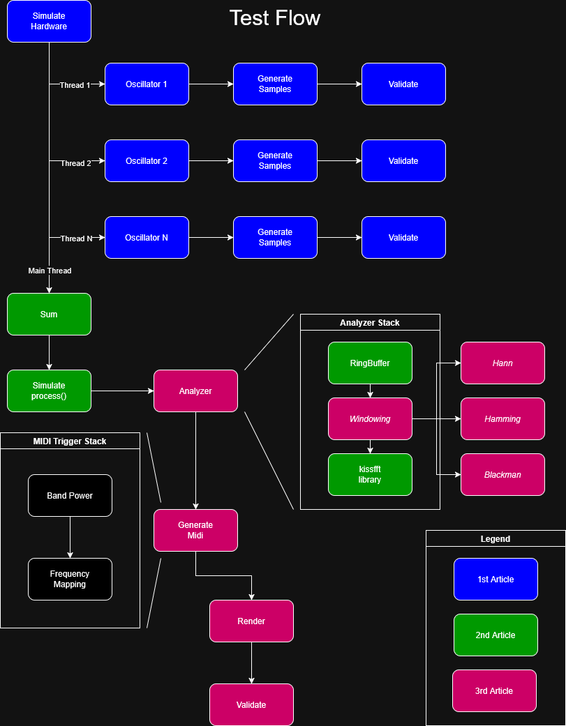
As you can see in the diagram, there is a lot to cover, we need to backtrack to cover the Windowing material that I didn't get a chance to cover in the last article.
Windowing
I currently have 4 windowing versions implemented. Mathematically, they're dead simple. But understanding them takes a bit more time. I'm more interested in discussing software and design than DSP, so I'll leave you with this article to fill in any gaps in knowledge: https://www.gaussianwaves.com/2020/09/window-function-figure-of-merits/
Window Design
The Window algorithm sits between the Wave Sum and FFT. Let's have a look at our implementation from the last post:
  std::span< const FPType > computeFFT()
  {
    // ensure our RingBuffer has enough data
    if ( !hasFrame() ) return {};

    // this is all we need to get the real & imaginary parts
    // from the library
    kiss_fftr( m_fft_cfg, m_sampleBuffer.data(), m_fftOut.data() );

    // now we need to get the magnitude
    setMagnitude();

    // return our result
    return m_magnitude;
  }
As you can see, we hand off our RingBuffer (m_sampleBuffer) directly to kissfft. If we design something, we want it to be seamless, such as in the following:
std::span< const FPType > computeFFT()
{
  if ( !hasFrame() ) return {};

  // apply window
  m_windowImpl.apply(
    m_sampleBuffer.data(),
    m_windowBuffer.data(),
    m_sampleBuffer.getCapacity() );

  // apply FFT
  kiss_fftr( m_fft_cfg, m_windowBuffer.data(), m_fftOut.data() );

  setMagnitude();

  return m_fftOutputBins;
}
Regardless of whether we want the Windowing algorithm to be hot-swappable, a templated member variable, or something else, we need it to conform to a standard interface.
The Window Interface
Let's look at a design first of how we want things to play together and then we'll start fleshing out the interfaces and implementations.

There are two things to note about the Windowing interface design:
- Each Window algorithm needs an initialization phase where it creates a precomputed buffer
- Magnitudes work slightly different after windowing, so we'll need access to a few options (namely, Coherent Gain and RMS Gain)
struct IWindowing
{
  virtual ~IWindowing() = default;

  virtual void initialize( const size_t szBuffer ) = 0;
  virtual void apply( const FPType * src, FPType * dst, const size_t szBuffer ) const = 0;
  virtual FPType getCG() const = 0;  // coherent gain
  virtual FPType getRG() const = 0;  // RMS gain
  virtual E_WindowingType getWindowType() const = 0;
};
Because I'm not a windowing expert and some windowing techniques may differ wildly from others, I'm going to implement an interface that all my APIs will use and then I'm going to implement a WindowBase because I don't want to copy and paste loads of boilerplate.
class WindowingBase : public IWindowing
{
public:

  WindowingBase() = default;

  void apply(
    const FPType * src,
    FPType * dst,
    const size_t szBuffer ) const override
  {
    // ensure the precomutation phase has been completed
    // and that our incoming buffer size matches expectation
    assert( m_isInitialized );
    assert( m_precomputedBuffer.size() == szBuffer );

	// all we do is multiply the raw buffer by the precomputed buffer
    for ( size_t i = 0; i < szBuffer; ++i )
      dst[ i ] = src[ i ] * m_precomputedBuffer[ i ];
  }

  // our gains
  FPType getCG() const override { return m_cg; }
  FPType getRG() const override { return m_rg; }

protected:

  // transform is a callback to a specific implementation that
  // transforms a sample we give it. we are able to calculate the
  // CG and RG based on what we get back.
  void initialize(
    const size_t szBuffer,
    std::function< FPType( const size_t ) > && transform )
  {
    m_isInitialized = true;
    m_precomputedBuffer.resize( szBuffer );

    // a sanity check
    if ( szBuffer < 2 )
    {
      std::cerr << "szBuffer is too small\n";
      m_precomputedBuffer.assign( szBuffer, 1.f );
      m_cg = 1.f;
      return;
    }

    // these are used in our gain calculations
    FPType sum        = 0.0f;
    FPType sumSquared = 0.0f;

    for ( size_t i = 0; i < szBuffer; ++i )
    {
      // call our transform callback
      m_precomputedBuffer[ i ] = transform( i );

      // CG
      sum += m_precomputedBuffer[ i ];

      // RG
      sumSquared += m_precomputedBuffer[ i ] * m_precomputedBuffer[ i ];
    }

    // Coherent Gain
    m_cg = sum / static_cast< FPType >( szBuffer );

    // RMS Gain
    m_rg = std::sqrt( sumSquared / static_cast< FPType >( szBuffer ) );
  }

private:

  bool m_isInitialized { false };

  std::vector< FPType > m_precomputedBuffer;

  FPType m_cg { 0.f }; // coherent gain
  FPType m_rg { 0.f }; // RMS gain
};
By having that base class, we have our specific implementations focus solely on the math formulas. Here's the Hann. The Hamming and Blackman are set up identically:
class HannWindowing final : public WindowingBase
{
public:

  void initialize( const size_t szBuffer ) override
  {
    WindowingBase::initialize(
      szBuffer,
      [ &szBuffer ]( const size_t i ) -> FPType
      {
        // w[ n ] = 0.5 * ( 1−cos( 2πn / ( N−1 ) ) ) = Hann
        return 0.5f * ( 1.0f - std::cos( TAU * static_cast< FPType >( i ) / static_cast< FPType >( szBuffer - 1 ) ) );
      });
  }
};
Windowing Output
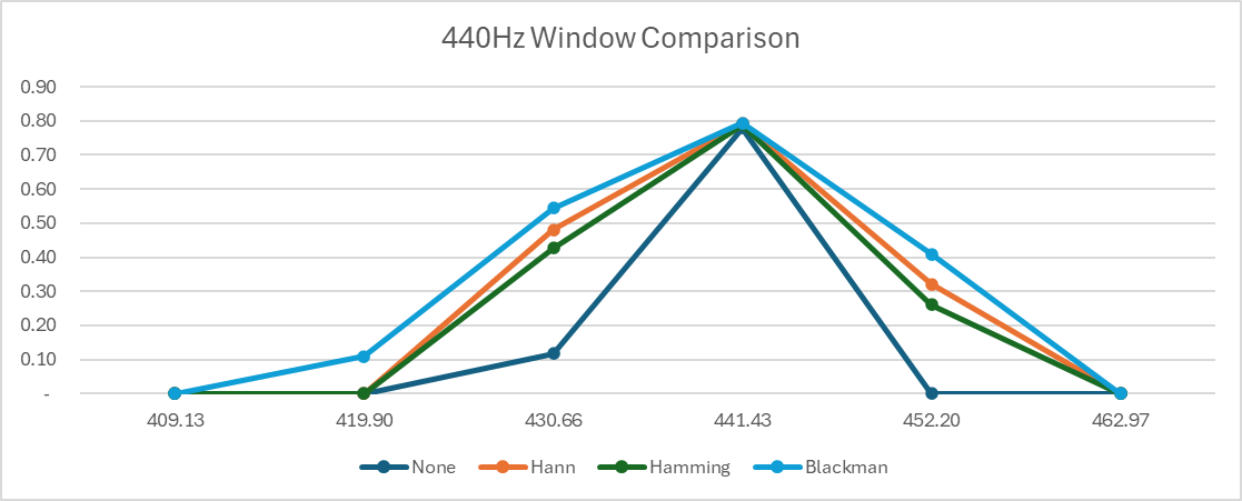
Let's take a look at something interesting now that might be counterintuitive. I ran this using all 4 options on identical data using the following setup:
440 Hz summed               A4
1046.5 Hz summed            C6
2637.02 Hz summed           E7
Sum Buffer Size: 220500

Ring Sections: 32           32 * 128 = 4096 Buffer Size
Ring Section Size: 128
Ring Hop Sections: 16       50% overlap in Ring Buffer

FFT Window Size: 4096
FFT Bin Size: 10.7666
Magnitude Threshold: 0.1    Any magnitude >= 0.1 will be printed

It looks like more leakage! What's actually happening is energy redistribution. Windows trade narrower main lobes for reduced side lobes. This becomes apparent in the graph below, showing energy around the 440 Hz mark.
Why FFT Bins Are Not So Good for Musical Purposes
FFT Bins are uniformly spaced, e.g., an FFT Window Size of 4096 with a sample rate at 44,100 means we'll get frequency bins of 10.76 Hz uniformly across the entire frequency band. But that's not how music works, since it's logarithmic.

Linear FFT bins (gray) vs logarithmically spaced MIDI note frequencies (blue)
At low frequencies, multiple musical notes fall within a single FFT bin. At higher frequencies, bins become overly dense relative to musical spacing. This mismatch is why raw FFT bins are not musically aligned.
To further bring the point home, have a look at C across different octaves.
| Note | Octave | Frequency |
|---|---|---|
| C | 0 | 16.35 |
| C | 1 | 32.7 |
| C | 2 | 65.41 |
| C | 3 | 130.9 |
| C | 4 | 261.6 |
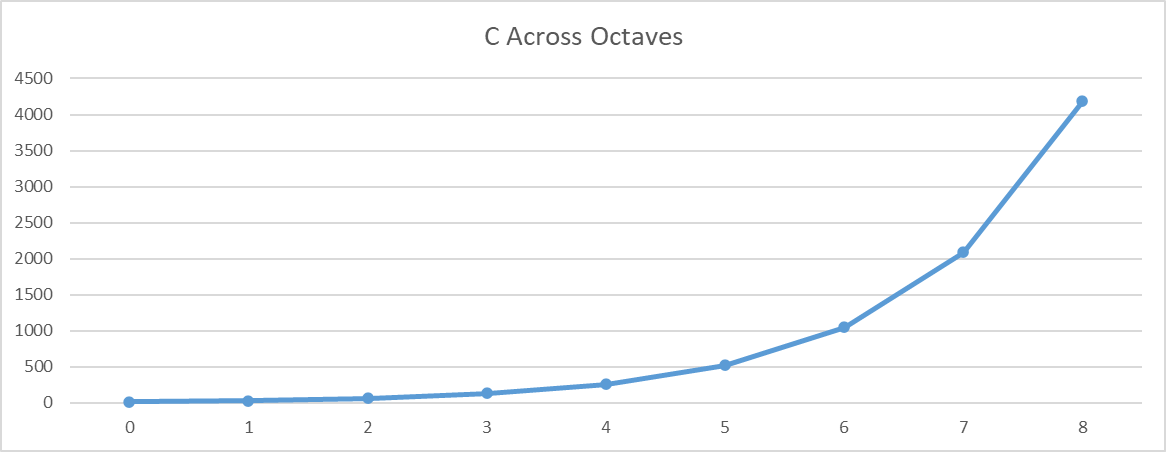
So the formula for a frequency across octaves is:
$$f = f_0⋅2^n$$
Moving from Bins to Notes
We've got a good starting point. So we'll keep doing the following:
- Generating waves
- Summing waves
- Windowing summed wave
- Running FFT
But here's where we're going to change things up. I want this to be a creative endeavor, where users can play around, so here's what I'm proposing:
- Group FFT bins into MIDI note grid
- Add harmonic reinforcement
- Primary Note = strongest energy
- Adjacent semitones = smaller energies
- Octaves = harmonic energy
- Neighbors = aesthetic bleed
All of those should be user-controllable.
Changing FFT Magnitude
Humans perceive loudness logarithmically (notice a pattern?), so that means we need to scale our raw magnitudes accordingly. In the last article, we played around with using:
$$mag = \frac{1}N \sqrt{r^2 + i^2}$$
Now we're going to use dB, which is a log scale and more natural way that users interact with frequencies.
$$dB=20log10(mag)$$
MIDI Mapping Frequencies
As discussed above, FFT bins are not musical. We lose information on the bass end of the spectrum because those notes are closer together. If our FFT bins are 10.7666, then we have the following:
| Bin Idx | Freq Range | Midi Pitch |
|---|---|---|
| 0 | 0 | |
| 1 | 10.7666 | 4 |
| 2 | 21.5332 | 16 |
| 3 | 32.2998 | 23 |
| 4 | 43.0664 | 28 |
| 5 | 53.833 | 32 |
| 6 | 64.5996 | 35 |
| 7 | 75.3662 | 38 |
| 8 | 86.1328 | 40 |
| 9 | 96.8994 | 42 |
| 10 | 107.666 | 44 |
| 11 | 118.4326 | 46 |
| 12 | 129.1992 | 47 |
| 13 | 139.9658 | 49 |
You can see that from 0 - 118.43 the MIDI notes can't be mapped 1:1. For example, C1 = ~16.35 Hz and Db = ~17.32, while Bin 2's range is from (10.7666 - 21.5332].
Options
- Option 1: Prevent FFT window sizes below 8192 and don't allow anything below 59 Hz.
- Option 2: Add harmonics with decreasing weights and make fundamentals win over harmonics
Option 1 is the easiest. On principle alone, I can't do it, though. It immediately violates our flexibility rule we stated at the start of this adventure.
Add Harmonics with Decreasing Weights
This took a bit of reading to understand, but I think I've got the hang of it. We need a scoring system that sits right on top of our FFT magnitudes that does the following:
- Band-sums around each note's expected frequency
- Adds harmonics (2f, 3f, 4f, ...) with decreasing weights so that fundamentals get a boost over the harmonics
There are some tweaks that we can do to fine-tune this too, which makes me more excited.
$$S(note) = \sum_{h=1}^{H}{ω_h}E(hf_{note}) $$
This has to do with harmonics and adjusting their values. If you need some background on fundamentals and harmonics, then this is an excellent video: https://www.youtube.com/watch?v=gT0IqL1dyyk
Setting Up Interfaces
We need to take in output from the FFT and because our FFT backend may change, we want to use an interface.
// we want our FFT bin to be flexible in what it provides
struct FFTBin_t
{
  FPType normalized     { 0.f }; // Coherent Gain applied
  FPType powerAmplitude { 0.f }; // Power Amplitude applied
};

struct IFFT
{
  virtual ~IFFT() = default;

  /// true whenever an FFT computation can be performed
  [[nodiscard]]
  virtual bool hasFrame() const = 0;

  /// resets the FFT's underlying buffer and any other state
  virtual void reset() = 0;

  /// adds a block of data to the current underlying buffer
  virtual bool processBlock(
    const FPType * samples,
    size_t szSamples ) = 0;

  /// Computes the FFT on the current underlying buffer. Will be empty
  /// if hasFrame() is false
  virtual std::span< const FFTBin_t > computeFFT() = 0;
};
And because we want to be able to swap out our Midi Mapper, we're going to align our input of the mapping process and then set a standard for the output:
struct FrequencyEnergyItem_t
{
  uint8_t midiPitch  { 0 };    // what's the midi pitch?
  FPType  energy     { 0.f };  // what's the energy of this midi pitch?
};

struct IFrequencyMapper
{
  virtual ~IFrequencyMapper() = default;

  // we consume the FFT input and provide our own output
  virtual std::span< const FrequencyEnergyItem_t >
    map( const std::span< const FFTBin_t > bins ) = 0;
};
Where We're Going Next
In Part 4, we'll:
- Implement harmonic scoring
- Explore band summation strategies
- Add weighting curves
- Compare detection stability across window sizes